Parallel Computing
Parallelising code is not always necessary and not always possible, but luckily this scenario is suitable to optimise, since from the mathematical model, the force calculation (gravitational interaction) will have a \(O(N^2)\) complexity, since all N particles must interact with all the rest, like in the following example:
for (int i = 0; i < Nact ; i++)
{
    for (int j = 0; j < N ; j++)
    {
        ...
        gravitational_interaction(i, j);
        ...
    }
}
CPU
First of all, we started implementing the mathematical model of the H4 scheme, without any kind of parallelism. Thanks to this simple situation, we are able to asses a simple test (1024 particles, evolved until the first N- body time unit) to see if the bottleneck is just the force calculation process, which after using a profiling, we checked it is.
time  seconds  seconds      calls s/call s/call  name
80.46    87.52   87.52 1296647743   0.00   0.00  gravitational_interaction(int, int)
11.44    99.96   12.44     799495   0.00   0.00  init_dt(float*)
 3.41   103.67    3.71     414230   0.00   0.00  save_old()
 3.04   106.98    3.31     414230   0.00   0.00  correction_pos_vel(float, int)
 0.96   108.02    1.04     414230   0.00   0.00  find_particles_to_move(float)
 0.70   108.78    0.76     414230   0.00   0.00  next_itime(float*)
 0.00   108.78    0.00     414230   0.00   0.00  get_energy_log(int, float)
 0.00   108.78    0.00     414230   0.00   0.00  update_acc_jrk(int)
 0.00   108.78    0.00     414230   0.00   0.00  predicted_pos_vel(float)
 0.00   108.78    0.00       2048   0.00   0.00  magnitude(double, double, double)
It is good to remember that the CPU was designed to have a good performance in parallel and non-parallel scenarios, because it minimises the latency experimented by a thread due to the large cache memory.
Once we detected our bottleneck, we can start trying different APIs, libraries, techniques to optimise our code.
OpenMP
A widely used API to parallelise code sections in an easy way is OpenMP, which is an API that provides a shared memory multiprocessing programming.
Since OpenMP implement multi-threading using a fork-join model we need to specify explicitly in the code the sections that will be parallel.
Parallelising for-loops is easy with OpenMP since there is a special pragma option for them:
#pragma omp parallel for
for (int i = 0; i < N ; i++)
{
    ...
}
This will split the N- loops into the available threads. There is no need of adding extra synchronisations statements or something similar, OpenMP will take care of it automatically.
Since we have a nested for-loop, we want to parallelise them in a sightly different way:
#pragma omp parallel for private(j)
for (i = 0; i < Nact; i++)
{
    ...
    #pragma omp parallel for
    for (j = 0; j < ns->n; j++)
    {
        ...
        gravitational_interaction(i, j);
        ...
    }
}
In this case, the private argument will allow every i- thread to have their own copy of the j variable, avoiding conflicts related to what is the current value of it (since all of the threads will try to change it value).
OpenMP is very simple, but has it costs, the speed-up and scaling it is not so significant compared to other specially written parallel code.
Preliminary results can be found in the section Preliminary results.
MPI
Moving on to a different approach, we have the case of Message Passing Interface (MPI), which as its name states, is a message-passing system which gives another type of environment to optimise our application.
Since one of the goals of MPI is to provide a communication protocol to communicate different nodes/computers, it is also possible to use in one machine, from where every core can act as a different node.
The inner for-loop of our implementation is always going up to N particles, compared to the outer which is going up to Nact particles, so makes more sense to focus the parallelization efforts in the inner one.
Our simulation is very simple, and it is based into splitting the j- particles from the inner loop among the available cores/slaves in the way that an i- particle will get the total force acting on it after a reduction of the preliminary calculations performed by the slaves over different j- particles.
This idea can be represented as:
for (int i = 0; i < Nact; i++)
{
    ...
    for (int j = j_ini; j < j_end; j++)
    {
        gravitational_interaction(i, j);
    }
    ...
}
where j_ini and j_end will be different for every salve
being use. A little example, lets consider N=800, and lets say we have 4 available
slaves, the distribution of this values will be:
- slave 1:
j_ini = 0,j_end = 200- slave 2:
j_ini = 200,j_end = 400- slave 3:
j_ini = 400,j_end = 600- slave 4:
j_ini = 600,j_end = 800
So, slave 1 will calculate the interaction of the i- particle with the j- particles \(0, 1, 2, ..., 199\), slave 2 with \(200, 201, ..., 399\), and so on.
After that we need to perform a reduction of the data, since we want the total force on the i- particle. Here we tried two different approaches, adding the reduction for every i- particle step and a general reduction after both loops were over.
- Reduction for every i-particle.
for (int i = 0; i < Nact; i++)
{
    ...
    for (int j = 0; j < N; j++)
    {
        gravitational_interaction (...);
    }
    ...
    MPI_Allreduce (...);
}
- Reduction of all the Nact i-particles.
for (int i = 0; i < Nact; i++)
{
    ...
    for (int j = 0; j < N; j++)
    {
        gravitational_interaction (...);
    }
    ...
}
MPI_Allreduce (...);
Preliminary results can be found in the section Preliminary results.
GPU
The Graphic processors (GPUs) are an important piece in the scientific computing scene, being a highly efficiency solution in terms of computational performance and energy consumption.
As programmable high-throughput parallel processors, the GPU have become in a new area in the High Performance Computing (HPC) world, due its capacity of being used in general-purpose computations.
Nowadays, the GPU spans in different aspects of the computation, from smallest cell phones or gaming devices, to largest super computing clusters around the world, including areas as computational visualisation, cloud computing, game development, etc.
Architecture
Before diving into the GPU architecture, we have to understand how the CPU works alone and how it works with a GPU.
To perform a certain operation on the CPU, the data and programs which lies in the RAM memory, travel through the data bus to the processor. The CPU has a very complex control unit, and really fast computing cores.
If we want a program that uses the whole CPU capacity we need a very complex program, even with the new technology. Another issue with the CPU computing, is the limitation of the data transfer between the RAM and the processor, being really slow. That is the main reason of the large cache memory that every CPU has, using an important area of the physical processor. The idea of the cache memory is to store the data temporarily, and use them to perform the computation.
In this scenario, the GPU appears as an external device to this RAM/CPU pair. communicating with the computer through the PCIe bus.
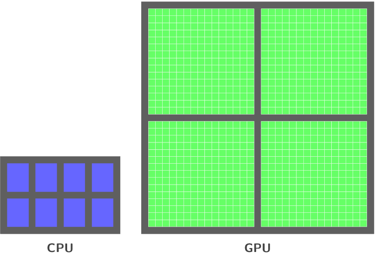
The big picture of the difference in terms of cores between the CPU and the GPU is described in the next figure:

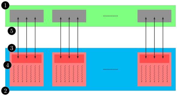
In simple words, the GPU is a multiprocessors array, each one of them has several cores, which execute a program concurrently, a synchronisation mechanism and shared memory. which can be seen in the next figure:

where each processor array has a cache memory and a control unit. Also the GPU has a RAM memory, which it is one of the different memories on the GPU, called global memory. This will be discussed in the next sections.
Flynn’s taxonomy
| Single instruction | Multiple instruction | |
|---|---|---|
| Single data | SISD | MISD |
| Multiple data | SIMD | MIMD |
The GPU is formed by Streaming Multiprocessors (SM), which is composed by several Streaming Processors (SP), also known as “GPU cores”.
The number of SP in each SM depends on the GPU architecture, for example in our case, we use NVidia Tesla cards, in which every SM’s are formed by 8 SP, and for example in the new Fermi cards, the SM are composed by 16 SP.
So, depending of this components, SM and SP, we have two different level of parallelism according to Flynn’s taxonomy, MIMD in the first case and SIMD in the second one, because we can execute different instructions for each SM but inside one of them, all the SP must perform the same task, this implies that the GPU exploits the data level parallelism.
Furthermore, it is important to understand the differences in the design and goals of the CPU and GPU. The CPU was designed to have a good performance~footnote{Capacity of perform individual instructions in a certain time} in parallel and non-parallel scenarios, on the other hand, the GPU was designed to do highly parallel work. Due the cache memory distribution in both chips, the CPU minimises the latency~footnote{Measure of time delay experienced in a system} experienced by one thread, and the GPU maximises the throughput~footnote{Capacity of perform a whole task in a certain time} of all threads.
CUDA
The Compute Unified Device Architecture (CUDA), is an extension of the C/C++ programming language which contains either a compiler as some development tools to write code that run on an nVidia GPU.
Programming CUDA applications implies writing code either in the CPU (host) and the GPU (device), which exhibit a large amount of data parallelism, an scenario that allows to perform some task simultaneously along the data, described in the previous section. The host code is simple C code, but the device code include some keywords to labelling parallel functions, this are called kernels.
Due CUDA threads are much lighter than CPU threads (a few clock cycles), it is not an issue to call large amounts of threads at some time, thanks to the efficient hardware support.
- Partition the data in subsets that fits in the shared memory.
- Handle each data subsets with blocks of threads.
- Load the data subset of the global memory in the shared memory.
- The idea is to perform the action using multiple threads to sue the memory level parallelism.
- Perform the calculation in each data subset of the shared memory.
- Copy the results from shared memory to global memory.
The execution of a CUDA application is described in the figure Typical CUDA programming strategy., which typically is a couple of steps between the host and the device.
Out current implementation is based in the j- parallelization idea presented by [NitadoriAarseth2012].
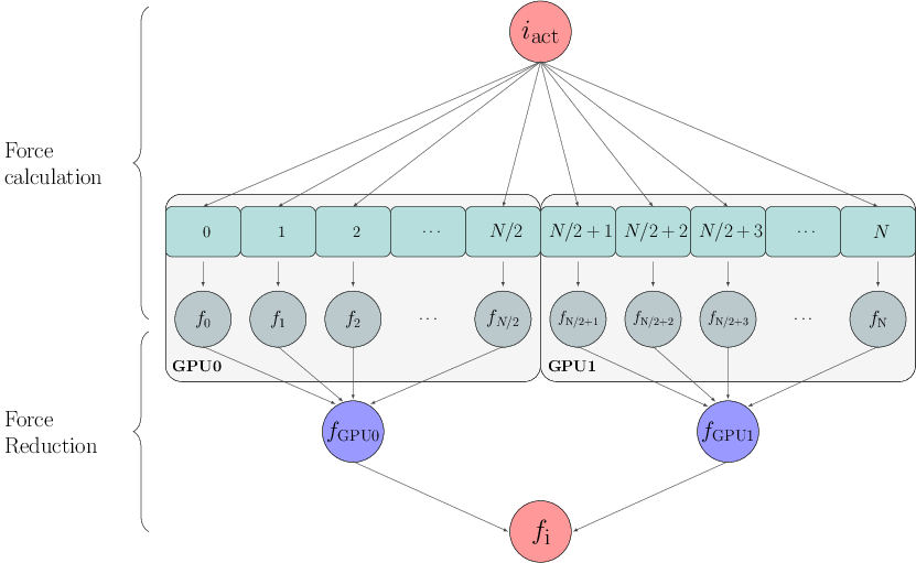
Our configuration is based in the idea presented in [NitadoriAarseth2012]. This parallelization scheme split the \(j-\) loop instead of the \(i-\) loop, in this case, we have two sections, the first is to calculate the force interactions of the \(i-\) particle with the whole system but by different threads, then a reduction (sum) is necessary to get the new value for the \(i-\) particle force.
Preliminary results can be found in the section Preliminary results.
| [NitadoriAarseth2012] | (1, 2) Accelerating NBODY6 with Graphics Processing Units http://arxiv.org/abs/1205.1222 |

