N-body integration
The Hermite 4th order integrator (H4) [MakinoAarseth1992] is a widely used N- body integrator scheme, which is used in the famous Aarseth integrator family [Aarseth1999] [Aarseth2003]. This integrator are useful as an starting point because:
- First of all, all Aarseth codes are published, so it is easy to compare new implementations, with an existing working code.
- The NBODY families are an evolution of a N- body integrator, so it is convenient to take a look of previous version, to understand determined process.
- The publications around Aarseth codes is enough to build up an idea of how its integrator works.
The H4 integrator scheme is based on a predictor-corrector scenario, this means, that we will use an extrapolation of the equations of motion to get a predicted position and velocity at some time, then we will use this information to get the new accelerations, then corrects the predicted values using interpolation, based on finite differences terms. We can use polynomial adjustment in the gravitational forces evolution among the time, because the force acting over each particle changes smoothly.
To predict the equation of motion, we have an easy to evaluate term, which is an explicit polynomial. This prediction is less accurate, but it is improved in the corrector phase, which consist of an implicit polynomial that will require good initial values to scale to a good convergence.
This algorithm it is called fourth-order, because the predictor consider the contributions of the third order polynomial, then, after obtaining the accelerations, adds a fourth-order corrector term.
Hermite 4th order
The mathematical formulation of the integrator main steps are the following:
Prediction,
Force calculation,
where,
is important to note, that \((\boldsymbol{v}_{ij}\cdot \boldsymbol{r}_{ij})\) correspond to the dot product, and not a simple multiplication.
Correction,
Calculate the 2nd and the 3rd derivative of the acceleration \((\boldsymbol{a}_{i,1}^{(2)}, \boldsymbol{a}_{i,1}^{(3)})\) using the third-order Hermite interpolation polynomial constructed using \(\boldsymbol{a}_{i,0}\) and \(\boldsymbol{\dot{a}}_{i,0}\):
where \(\boldsymbol{a}_{i,0}\) and \(\boldsymbol{\dot{a}}_{i,0}\) are the acceleration and jerk calculated at the previous time \(t\), the second and third acceleration derivatives \(\boldsymbol{a}_{i}^{(2)}\) and \(\boldsymbol{a}_{i}^{(3)}\) are given by:
where \(\boldsymbol{a}_{i,1}\) and \(\boldsymbol{\dot{a}}_{i,1}\) are the acceleration and the jerk at the time \(t_{i} + \Delta t_{i}\).
Finally, it is necessary to calculate the next time-step for the \(i\) particle (\(\Delta t_{i,1}\)) and time \(t\) using the following formulas:
where \(\eta\) the accuracy control parameter, \(\boldsymbol{a}_{i,1}\) and \(\boldsymbol{\dot{a}}_{i,1}\) are already known, \(\boldsymbol{a}_{i,1}^{(3)}\) has the same value as \(\boldsymbol{a}_{i,0}^{(3)}\), due the third-order interpolation; and \(\boldsymbol{a}_{i,1}^{(2)}\) is given by:
Block time steps
The main idea to use block time steps is to have several blocks (group) of particles sharing the same time steps, this will decrease the amount of operations of the integration process obtaining a similar accuracy than the individual time steps scheme.
In this scenario, the parallelization fits very good because compared with the individual scheme, we can have several chunks of threads working with different particles blocks.
The particle \(i\), will be part of the lower \(n-\) th block time step, between two powers of two quantities,
where \(\Delta t_{i}\) is determined by equation (1), and \(\Delta t_{s}\) is a constant.
The distribution of the particles among the blocks is determined by the following condition,
noindent and is described in the Figure~ref{fig:block_time steps}.
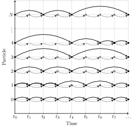
Block time steps illustration.
The different blocks are represented by different colours. Each particle is predicted (not move) at every time \(t\) (gray arrows), even if it’s not their block time-step (blue circles). The particles will be updated (moved) only in their block time-step (black circles). At every time that a particle is updated, they can change its block time-step, in this case, the particles \(1, 4\) and \(N\) change their block.}
For the boundaries of the time steps, we use the Aarseth criterion [Aarseth2003] for the lower limit,
where \(\eta_{I}\) is the initial parameter for accuracy, which is typically \(0.01\); \(R^{3}_{\rm cl}\) is the close encounter distance; and \(\bar{m}\) is the mean mass.
Typically \(\Delta t_{\rm min} = 2^{-23}\). On the other hand, we set a maximum time step \(\Delta t_{\rm max} = 2^{-3}\). When updating a particle’s time-step, if it is out the this boundaries, we modify the value to \(\Delta t_{\rm min}\) if \(\Delta t < \Delta t_{\rm min}\), and to \(\Delta t_{\rm max}\) if \(\Delta t > \Delta t_{\rm max}\).
| [MakinoAarseth1992] | On a Hermite integrator with Ahmad-Cohen scheme for gravitational many-body problems http://adsabs.harvard.edu/abs/1992PASJ...44..141M |
| [Aarseth1999] | From NBODY1 to NBODY6: The Growth of an Industry http://adsabs.harvard.edu/abs/1999PASP..111.1333A |
| [Aarseth2003] | (1, 2) Gravitational N-Body Simulations http://adsabs.harvard.edu/abs/2003gnbs.book.....A |